TL;DR

• The Yellow Jackets are a spectacular countrywide social protest movement that was active for months in 2018/2019;
• As a reaction to the protests, the French government organised a nationwide public debate to discuss important political issues;
• The protesters replied by launching their own online platform, where anyone could propose free-form demands or criticism and put it up to vote;
• This is a semantic analysis of that database.

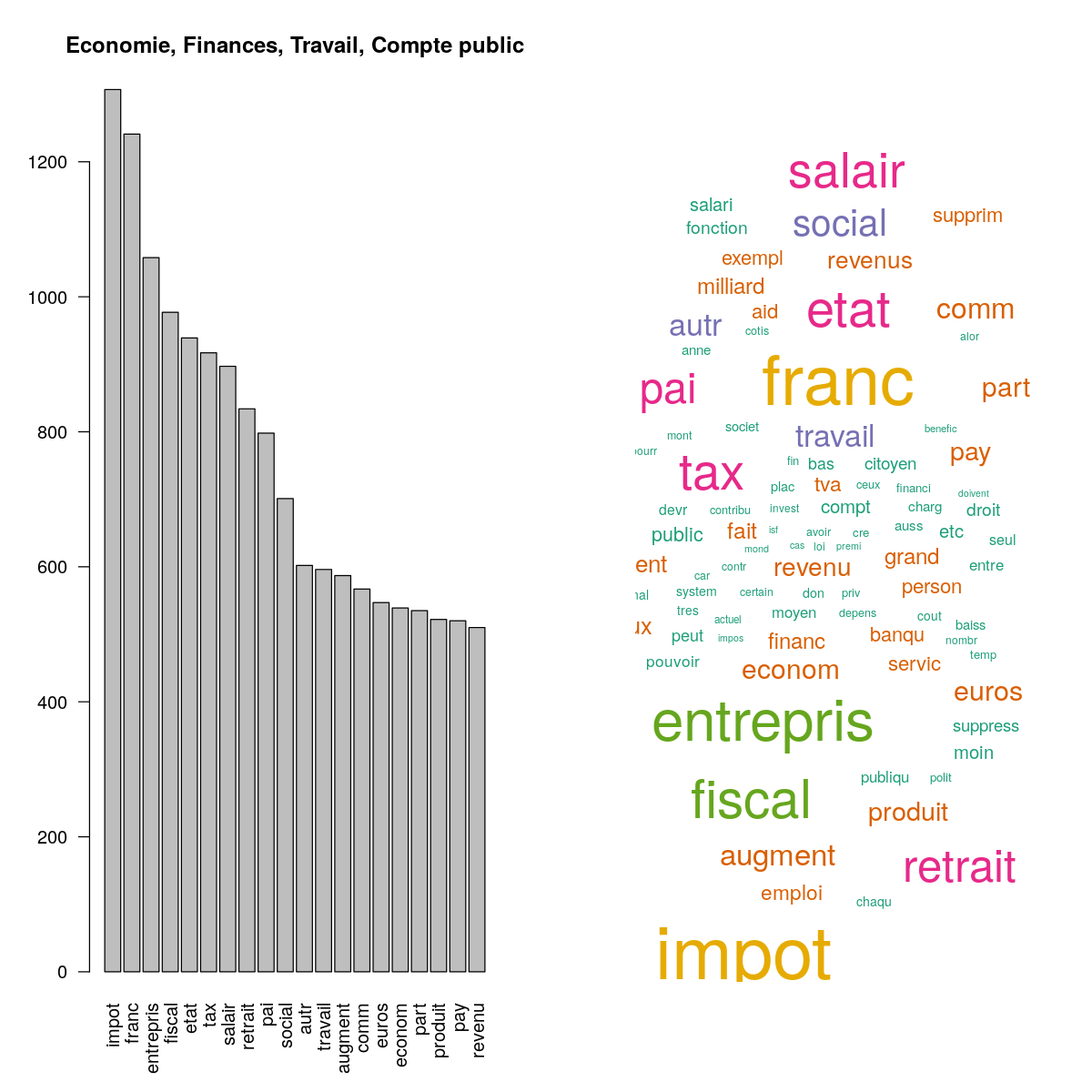
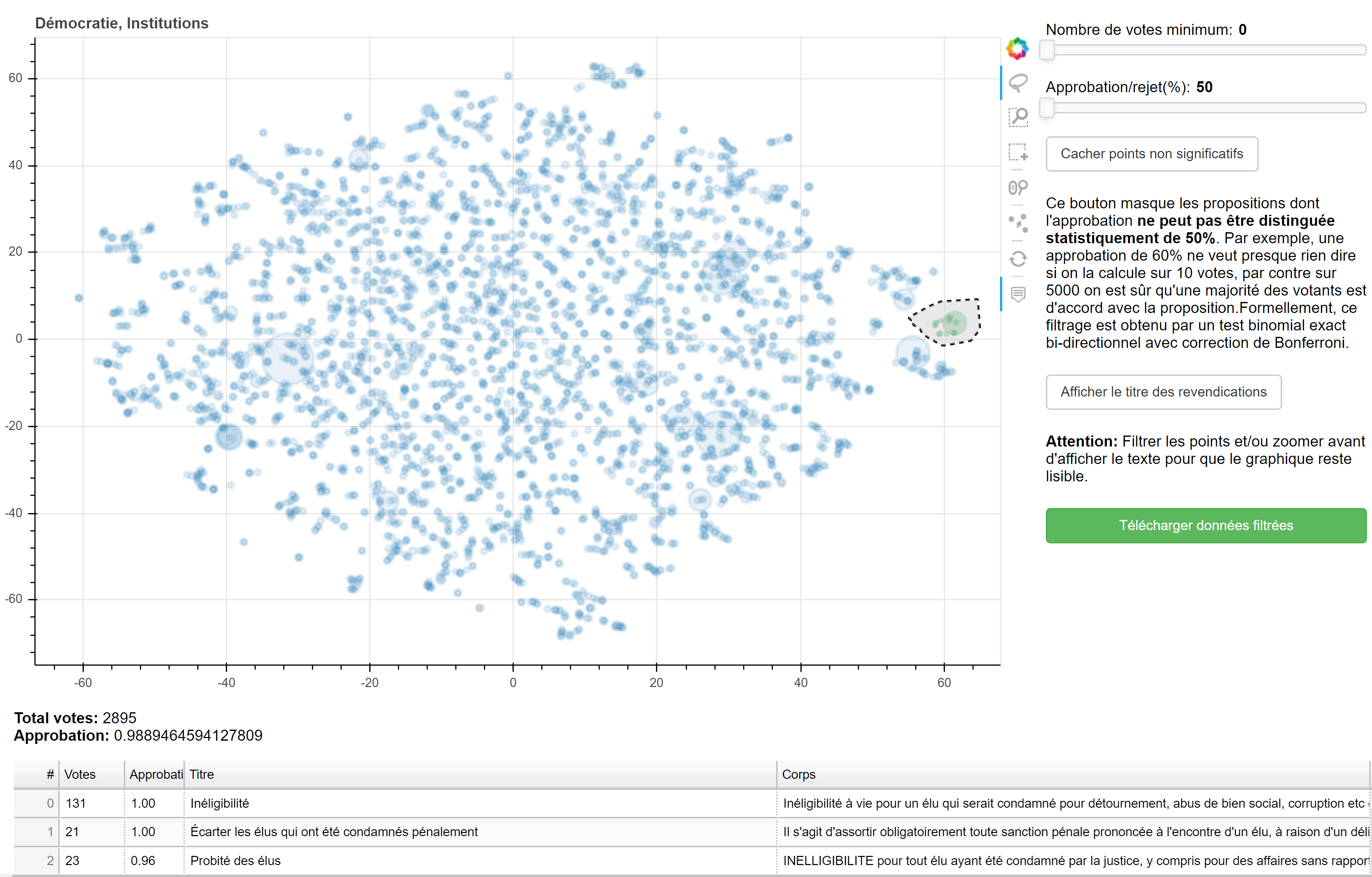
The main outputs of this analysis were navigation tools organised by broad social theme. One example, which covers “Democracy and Institutions”, is available here

The full analysis pipeline, as well as the remaining tools and a documentation (in French) are available on my GitHub page.

Introduction

For a couple of months in winter 2018-2019, the Yellow Jacket protests rocked the French political landscape. Composed of mostly working-class protesters from disinherited areas of peri-urban and rural France, the country-wide demonstrations took place every Saturday, forcing the government to back down on several reforms, and leading to an exercise in organised grassroots democracy dubbed the “great national debate”.

The protests organised organically on social media, had no clearly defined leader, and covered a very broad range of demands. Media struggled to cover the events, focusing either on clashes with police and property damage on the margins of the protests, or on a narrow set of “representative” demands extracted from protesters through street interviews. Since all attempts by the government to organise roundtables with organisers failed, no serious synthesis of the protesters’ demands was ever undertaken.

Mindful of the scale of the dissent, the government moved to clarify popular sentiment by organising what it called the “Great National Debate”. This was an ambitious plan to empower bottom-up democracy through citizen participation. It consisted of a form with very precise questions about specific aspects of interior and foreign policy. Undoubtedly, concerns over data complexity guided this choice, since answers to focused questions are much easier to mine than free-form text. Many people, however, felt disappointed by the platform, not the least of which the Yellow Jackets themselves, many of whom dubbed it too restrictive.

They then went on and contracted the same company who had won the government tender for the website of the Great Debate, and created “le Vrai Débat” (the True Debate). Its main characteristic was that it was exclusively free-form. Users could sign up, put forward a proposal, and other users would vote in favour or against. I learned about this endeavour on the radio and heard they were looking for analysts, so I contacted the organisers who granted me access to their database. This post is a walkthrough of the analysis.

Method

The full analysis protocol is documented on github in the form of Jupyter Notebooks. Unfortunately, they are mostly in French, as I had to document this for my French-speaking client. But here are the main steps in a nutshell:

Preliminary analysis

This was my first contact with text mining, so there was a lot of trial and error, exploratory analyses, and reading going on in the first few days of the project. But that allowed me to get a good grasp of the basic structure of the data.

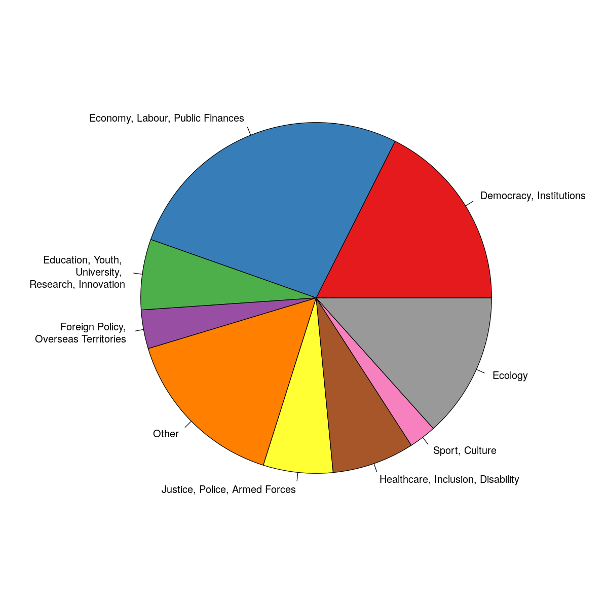
Most proposals were self-classified in the Economics and Public Finances, Democracy and Institutions, as well as Ecology categories. The latter is perhaps surprising, since the green transition was not thought to be a particular matter of concern to the Yellow Jackets, mostly a social protest movement.

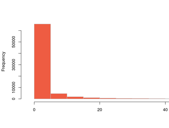
The dataset comprised 25,699 proposals with a very wide length and complexity: from “Referendum” or “Art everywhere” to the full outline of a constitution featuring more than 4,000 words. The distribution above has a fat right tail, and 95% of all proposals were less than 50 words long.

It was also obvious that the proposals would be difficult to interpret, because of the many spelling mistakes and neologisms present in the dataset. On top of that, many of the texts contained links, or were constituted of several proposals instead of one. This was clearly a difficult dataset.

At this point, it became clear from my reading that there were two approaches to analysing text data: the traditional one, where you try to clean your dataset as much as possible to make it understandable by a relatively rigid algorithm, or the modern one, where you directly cram your whole dataset into a very flexible one, such as a neural network (NN). Since I wanted to learn the basics, I went for the first option, which required a deep cleaning of the dataset.

Incorporating votes

The website’s voting system was not well-designed. It had a typical “social media” approach, which promoted already popular proposals by making them more visible. This increased the chances that some of them would become “viral” and others would be essentially forgotten. In my opinion, this was a serious design flaw, especially for a website that aimed to enable participatory democracy and give a voice to a perceived “silent majority”.

This is reflected in the distribution of votes:

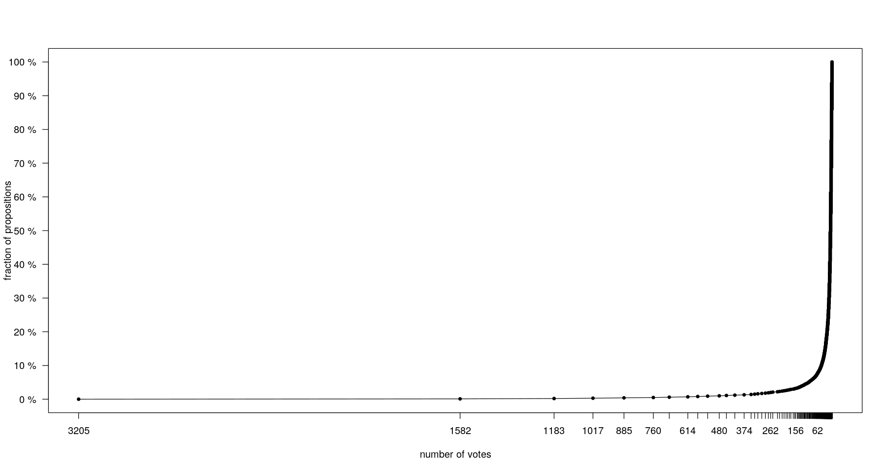
A consequence is that any approach focused on examining only the most voted proposals will explore only a tiny fraction of the diversity of opinions put forward by users. Another question is how representative such an approach would be:

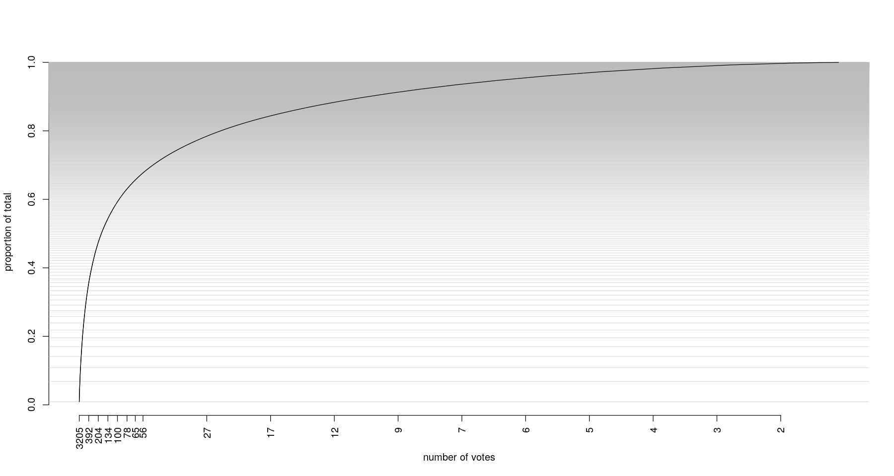
Sorting proposals by vote count and working your way down is actually a very unsuitable approach. The top 10 votes represent only 6% of all total opinions. To reach 80% of all cast votes, you would have to examine 2,220 proposals. Analysing the first 1,000 proposals, which is the approach chosen by Laboratoire Triangle, which also worked on the data, will represent 67% of votes and 8% of all proposals.

Approval rate

Looking at approval rates is interesting, since the movement had often been portrayed as incoherent or even contradictory. One option for considering a proposal approved/rejected is to set an arbitrary threshold in terms of number of votes and proportion approved/rejected. While this is easy to do, it ignores statistical power, which is really what we’re talking about here. Briefly, you want to exclude proposals where you can’t decide if the approval rate is significantly different from 50% (which corresponds to full ambivalence). We can calculate this very easily (see dashed lines below).

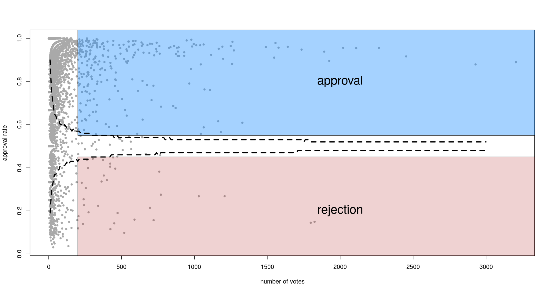
Most proposals actually fall above the top line or below the bottom one, which means they are well-powered to determine approval or rejection by the majority. There is also a higher number of approved than rejected proposals, which provides additional evidence towards a globally coherent political discourse.

From this data, it is clear that every effort should be made to be as inclusive as possible in the analysis. This means actually grouping similar proposals together by semantic proximity, so as to capture both the wide spectrum of ideas posted on the forum, and a high number of votes.

Quality control

Basic filtering

We start by removing links, web addresses (another option would have been to follow them and incorporate the text) and HTML tags, and by removing stop words. These are words that are uninformative from a semantic point of view (the, to, and, with), but that provide context to a human reader. I assume this is typical of non-NN methods where grammatical context is ignored.

The proposals are also split into a title and description. Either one or the other can be empty, especially for short proposals, so we paste them together.

We also convert all the corpus to lower case and remove common words that are not stop words but also relatively uninformative (such as “other”, “do”, and others).

Stemming

Stemming facilitates the analysis by removing affixes that make subtle changes to the meaning of a word (reclaimed becomes claim). Unfortunately, it sometimes makes things harder, not clearer, especially in languages with lots of close homonyms. Words with different meanings but similar spelling get chunked together in the same stem, losing a lot of semantic granularity:

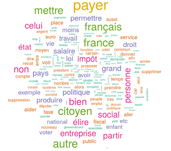
In the wordcloud above, note the two stems “fonction” and “person”. They exemplify the limits of stemming: the former could be the result of “fonction” which can mean function or role, or “fonctionnaire”, which means public servant. Similarly, the latter could come from “personne”, which both means a person and nobody, or “personnel”, which both means personal (adjective) or, well, the personnel (e.g. of a hotel). Another problem with this approach is that it can be hard to get a clear meaning from these visualisations when they only involve truncated words. A better option is lemmatisation.

Lemmatisation

In natural languages, words rarely remain constant. Verbs, for example, are conjugated (he was, I am), without changing the fundamental meaning of the word. This fundamental form, called a lemma, is crucial for grouping together words by meaning for text analysis. The degree of this morphological variability differs greatly between languages. Compared to English words, French ones are highly variable, since it is a gendered language, where every adjective will change its ending depending on the gender of the word it qualifies. In terms of linguistics, English is an analytic language, where relationships between words are mostly conveyed by small helper words ( with, her, will, would, shall), whereas French is a synthetic fusional language, where words change their forms to indicate these relationships. In this context, lemmatisation (finding the correct lemma for each word) is a fascinating problem, and one that often cannot be solved exactly due to the structure of language itself. For example, the French word “sort” can both be a conjugated verb (he/she/it exits) or a noun (fate). Without studying context, it is impossible to know whether it’s better to lemmatise it to “sortir” (to exit) or to leave it as is. When in doubt, the lemmatiser will report all equiprobable lemmas. Lemmatisation can be further informed by part-of-speech annotation, which determines the semantic class of a word. For example, “sort”, if assigned the “verb” class by a POS tagger, has a single unambiguous lemma.

There has been recent research into so-called context-aware lemmatisation, which draws on the meaning of the wider sentence to achieve better performance (unsurprisingly, using neural networks).

Spell-checking

In addition to better lemmatisation of known words, context-aware lemmatisers also produce better results for unseen words (particularly present in Internet corpora), such as “soz” instead of “sorry”, or spelling mistakes (e.g. “avaliable”).

There is an almost permanent debate in France about language. On the one hand, linguistic conservatives fret that recent generations are losing the capacity to express themselves properly, whereas progressives push for a simplification of French. Reforms were recently put in place to make a lot of the accents and complicated spellings optional in school curricula. This has not permeated through to data analysis tools however, so we need to spell-check our dataset for proper old-school French.

Context-unaware spell checkers suffer from the same limitations as lemmatisers. For example, “hel” is equally likely to be a misspelling of “hell” and “help”.

We use the HunSpell spell-checker, which is used in OpenOffice, Firefox and Chrome. This package is very restrictive, even considering words that are missing accents as wrongly spelled. For every spelling mistake, Hunspell makes suggestions.

Some spelling mistakes will be recurrent, those can correspond to abreviations. For example, one of the key demands of the Yellow Jackets was the “RIC”, abreviation for “citizen initiative referendum”. We identify the top 50 recurring mistakes and replace them by their corrected counterparts.

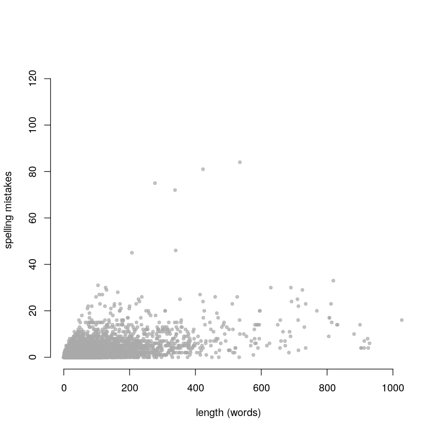
From the graph above, we see that the propensity to spelling mistakes falls into two groups. The first has a mistake/word count ratio of about 2% and contains most responders. The other is smaller but exhibits a much higher rate, at 16%. Examination of high-mistake, high-word count proposals confirmed a higher than average number of mistakes, perhaps indicative of a language processing condition such as dyslexia.

We now have a lemmatised, spell-checked corpus. Let’s try and cluster our proposals into semantic groups.

Information retrieval using tf-idf

In order to do that, we need to represent our documents in a space that will make clustering easy. The simplest way is to use the bag-of-words approach, which just counts how many times any given word appears in a document. Term Frequency-Inverse Document Frequency (TF-IDF) expands that approach by inverse-weighting those counts by their frequency across the whole corpus. The more frequent a word (think “because”, or “be”), the less important it is to the meaning of the sentence. A good description of these 2 approaches can be found here.

We then prune the dataset to exclude the least informative (most common across corpus) words. The pruning threshold is somewhat arbitrary, we use 0.99. Then we create a similarity matrix using the sim functions provided by text2vec. This allows us to do some very simple hierarchical clustering:

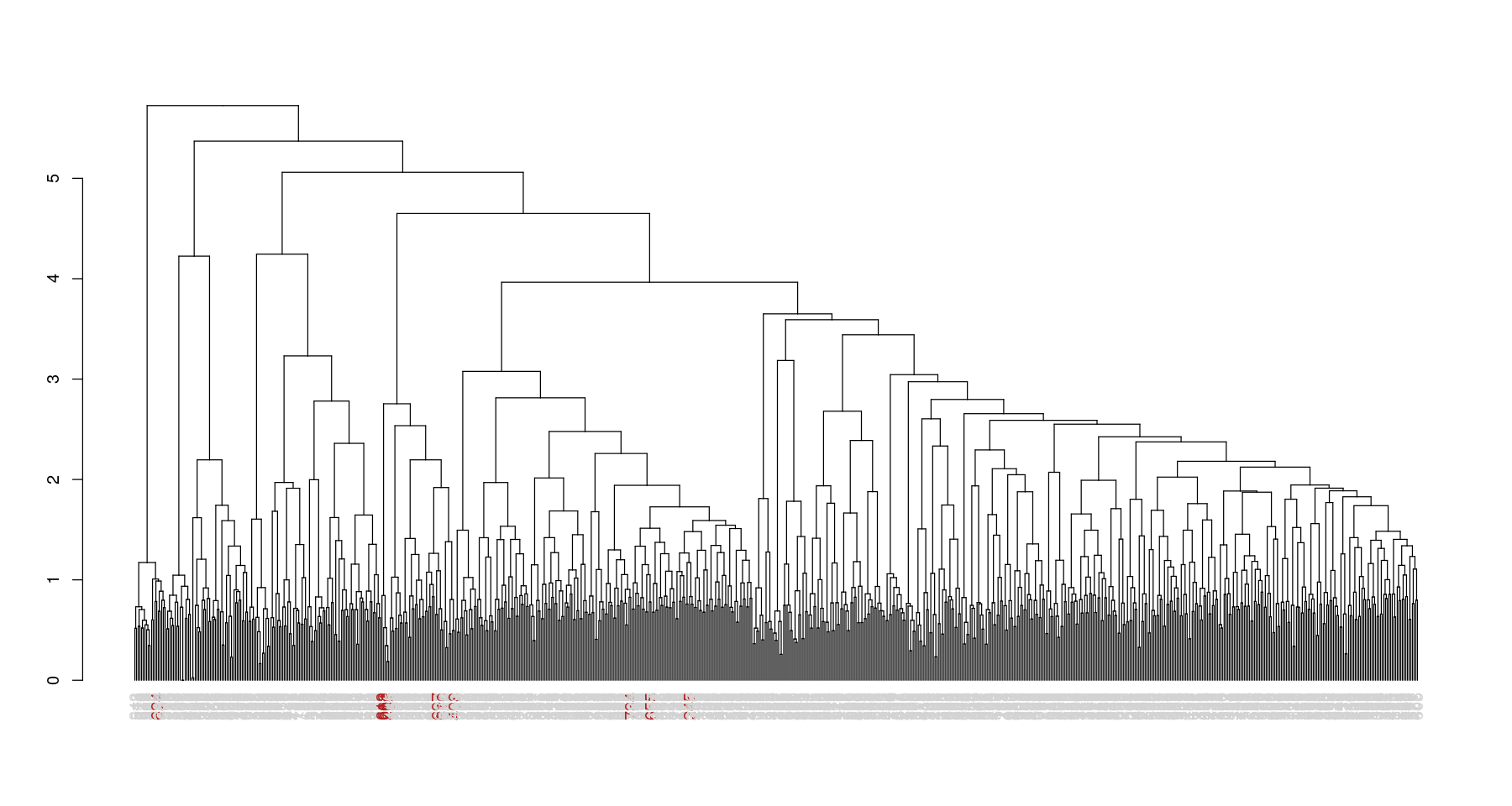
I chose to focus on “death penalty”, since it is extremely specific. Documents mentioning it are coloured red in the dendrogram above. The clustering does a pretty good job of aggregating most of the proposals, but a couple seem misclassified. Looking in more detail, the misclassified proposals are multi-topic, for example “stop immigration, deport foreign criminals, reinstate death penalty for terrorists”. In that latter case, the presence of the word “terrorist” was considered more specific than “death” and it got clustered in the terrorism cluster. Clearly, a similarity matrix does not capture the semantic complexity of this dataset. We must allow a document to belong to several clusters, i.e. have several topics.

Topic modelling with Latent Dirichlet Allocation

A useful method in this scope is latent Dirichlet Allocation. In a nutshell, it assumes that every document will be focused on a small number of topics, and that a small number of keywords are strongly specific to each topic (e.g. “death+penalty” or “president+impeachment”).

The main drawback of this method is that, similar to k-means, a specific number of topics to be modelled needs to be specified a priori. Fortunately there are ways to try and determine the best k (keeping in mind usual considerations about overfitting and holdout sets). We restrict to the “Justice, Police, Armed Forces” theme, which allows us to restrict our search space, and calculate multiple fit metrics for each k in a range. The metrics and the function used are described here.

This allows us to pinpoint the actual number of topics relatively precisely (around 21 in this case). However, I found that number to vary massively depending on the hyperparameters of the model. Notably, repeating the same tuning procedure with \(\LARGE\alpha=0.05\) gave an optimal \(\LARGE k=30\), which is 50% more than the previous procedure.

Moreover, both k led to numerous misclassifications. Proposals about the death penalty were classified with one advocating the criminalisation of perjury, and documents about legalising cannabis were grouped together with ones about creating a national DNA database. Overall though, LDA proved to be an accurate, if not very precise, aggregation method. The notebooks have a bit more exploration around multi-topic proposals, however this method definitely deserves more attention, as does CTM, a related method.

Word Embeddings

The last method I tried in my efforts to more closely map the granularity of this dataset was a more recent one. Word Embeddings are described in a nice paper here.

Briefly, word embeddings are representations computed using neural networks, that project words in a semantic space. The typical example from that paper is quite illustrative:

the result of a vector calculation vec(“Madrid”) - vec(“Spain”) + vec(“France”) is closer to vec(“Paris”) than to any other word vector.

Improvements described in the paper allow to model several linguistic quirks, such as the fact that “Air Canada” should be closer to “airline” and “PanAm” than “Montreal” or “Atmosphere”.

The main difficulty of applying such an algorithm is that the NN needs to be trained on a large corpus. The Yellow Jacket database is nowhere near as big to perform reliable inference, let alone usign hold-out or cross-validation.

Fortunately, there are plenty of pre-trained NNs around, although I’m lucky this was in French (finding a model would probably have been much harder if these protests had happened in Hungary or Dubrovnik!). I used the amazing dataset provided by J-P Fauconnier, trained on 1.6Bn words using the methods from the paper above.

The resulting model gave excellent results. Visualising the mapped dataset using t-SNE (an improved dimension reduction technique, compared to PCA) produced a cloud of small clusters, each very homogenous in semantic terms. This method correctly identified both the cannabis/drug legalisation cluster and the death penalty one.

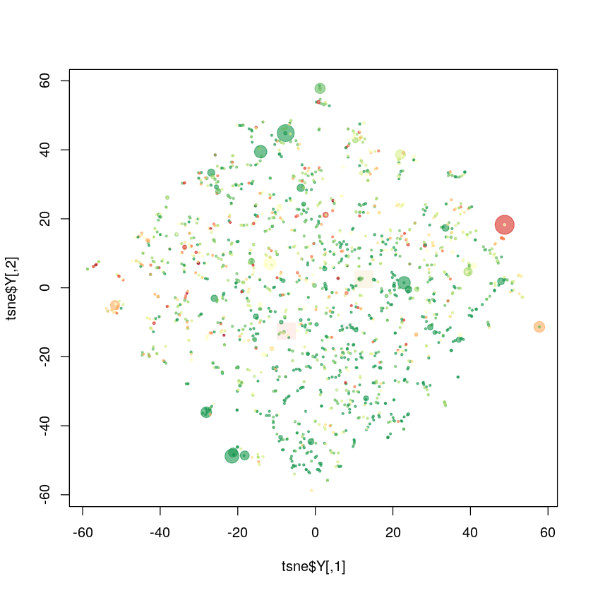
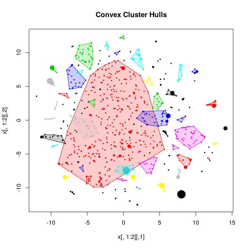
The issue now is to actually automate cluster creation, which is an issue that I unfortunately did not manage to solve given the tight timelines imposed by the Vrai Débat team. I got mixed results from DBSCAN, which may have been because the method is quite sensitive to its \(\LARGE\epsilon\) parameter, which determines cluster extension. This is definitely something that would require more investigation.

Elbow Grease

At that point I had a very good representation of the dataset using Text2Vec, a rough estimate of the number of topics from LDA, but no clustering method to produce a list that would capture most of the semantic variance in the dataset.

So I quickly put together a form of semantic explorer, which basically allows users to browse the t-SNE projected Text2Vec embeddings, display the content of the associated proposals as well as their approval rate. This was done using bokeh, an extremely powerful, yet chaotically maintained python library that i kind of have a love-hate relationship with. Using this browser, it should be possible to aggregate the greatest part of a dataset within a few hours.

Future directions

The issue with the current approach is that is is quite manual. This is due to two outstanding problems:

• I did not find any reliable clustering method, possibly due to the high granularity of the dataset;
• Clustering in any case will be sentiment-independent, which means that although a proposal and its opposite would be close to each other in the representation above, votes cannot be aggregated without taking sentiment into account.

The first point could probably be ameliorated with more investigation. For example, further tweaking the DBSCAN parameters, or using something more modern like the BIRCH method. Or even something specifically tailored for modelling many small, very dense clusters.

The second issue can be addressed with sentiment analysis, which basically computes a probability that a given document expresses a positive, negative or neutral opinion. With that annotation, approval rates for negative opinions could be complemented and automatically aggregated.